Predictions off Unpredictability
I’ve spent a lot of time being annoyed at missing data in healthcare.
Patient monitoring streams that drop out for hours. Vitals that come in bursts. Labs that appear once every few days. EHR time series that look like someone took scissors to them.
For years my mental model was:
“Okay, just clean it, impute it, then throw a decent ML model at it.”
And then I started playing with world models / JEPA-style ideas and realized:
that mental model is deeply incomplete.
This post is me unpacking that journey:
- why my first world-model demos totally failed
- what finally worked (the Seq2Seq imputation demo available at the end)
- and why a traditional ML model really can’t just “look at a larger slice” and magically match a world model—especially in healthcare.
1. My real problem: healthcare data is a mess
In healthcare, almost every time series is:
- irregularly sampled
- multivariate
- and full of missing values
ICU vitals, ward monitoring, RPM, EHR event streams—missingness is the rule, not the exception. Reviews of EHR-based modeling repeatedly call missing data one of the central challenges in clinical ML. Science Press Journal+1
People have tried all the classic fixes:
- last observation carried forward
- interpolation or smoothing
- simple statistical imputation
- more sophisticated multiple imputation (MICE)
- pre-imputing then training LSTMs or other deep models on the “completed” data PMC+1
But in practice, I kept seeing the same thing:
The more I tried to “pre-fix” the data, the less I trusted anything downstream.
At the same time, I’m reading about world models and JEPA and thinking:
These things are literally designed to handle partially observed worlds. Why can’t I get a tiny version of that working on a simple healthcare-style signal?
2. My failed “Hello World Model” attempts
I started where every blog post starts:
- a moving dot on a line
- a sine wave
- a point moving in a circle
- even a logistic map (chaotic system)
The plan:
- Build a “traditional” predictor (MLP / simple time-series model).
- Build a “world model” (encode → predict latent → decode).
- Mask or corrupt some observations.
- Show that the world model is robust, and the MLP falls apart.
In practice, what happened:
- On simple worlds (moving dot, circle), the MLP did great and the “world model” didn’t look better—sometimes it looked worse.
- On harder worlds (chaotic maps, noisy dynamics), the tiny “world model” collapsed—flat lines, diverging outputs, or general nonsense.
It took me a while to admit it, but the problem was conceptual:
I was calling something a “world model” that wasn’t really a world model.
I was basically taking an MLP, inserting an encoder and decoder, and hoping that would magically give it temporal memory and robustness.
It didn’t.
3. What is a world model, anyway?
In the literature, a world model is usually:
- some recurrent/structured model of the environment
- trained (often self-supervised) to predict future states or representations
- with a persistent internal state that summarizes what it has seen so far
The classic example is Ha & Schmidhuber’s World Models paper: they train a variational autoencoder + recurrent network to model RL environments, and then learn policies that operate inside that learned world. arXiv+1
JEPA (Joint Embedding Predictive Architectures, like I‑JEPA and V‑JEPA) takes a similar spirit but works in representation space: from one context patch, predict the representations of masked/held-out patches, without ever trying to reconstruct pixels directly. Meta AI+1
The common thread:
- They predict in latent space
- They maintain state over time
- They are trained on sequences with masking / context / targets
My early “world models” were none of those things. They were just slightly overcomplicated next-step regressors.
4. The demo that finally worked: Seq2Seq imputation
What did work is the example you’ve just been running:
- A smooth 1D signal (sinusoid + harmonic)
- 60% of the points randomly masked (set to missing)
- Two models:
- Traditional ML: MLP that predicts the next value from the last 5 inputs
- World model: a Seq2Seq LSTM that sees the entire corrupted sequence and learns to reconstruct the full clean sequence
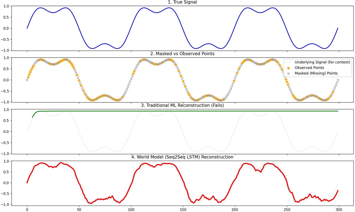
Visually, in the 4-panel plot:
- Panel 1 – True signal: a smooth wave.
- Panel 2 – Masked vs observed: orange dots (observed), grey X’s (missing).
- Panel 3 – Traditional ML reconstruction: noisy, jumpy, fails across long gaps.
- Panel 4 – World model reconstruction: smooth, follows the true curve across missing spans.
That’s the first time I got a “Hello World Model” demo that felt honest and non-gimmicky.
Under the hood:
Traditional MLP
- Input: a 5-point window
[x_{t-4}, …, x_t] - Target:
x_{t+1} - Trained only on positions where
x_{t+1}is not missing. - At inference, we roll it forward: each new prediction is fed back in.
Limitations:
- Only ever sees local slices of the signal.
- No persistent hidden state.
- When data are heavily masked, those 5 points are often mostly zeros or noise.
- Errors compound when we roll it forward.
Seq2Seq LSTM “world model”
- Encoder LSTM reads the entire masked sequence.
- Its hidden state learns a global summary of the signal’s shape.
- Decoder LSTM reconstructs the sequence step-by-step, trained with teacher forcing (it sees the real noisy inputs and learns to output the clean version).
- Loss is computed over the entire sequence, not just one-step fragments.
This isn’t JEPA in the strict research sense (we’re reconstructing in observation space, not purely in latent embeddings), but architecturally it’s much closer to a world model than the earlier toy networks:
- It has temporal memory
- It’s trained on full trajectories
- It learns a latent state that captures the shape of the process
This pattern—Seq2Seq + RNNs / attention for time-series imputation—is also exactly what’s appearing in the time-series imputation literature. PMC+1
5. “Can’t a traditional model just use a bigger window?”
This was my next question too.
If 5 points isn’t enough, why not 50? Why not 200?
Here’s why “just make the window bigger” doesn’t solve it.
5.1. Bigger windows mostly give you more missing values
With 60% missingness:
- In a 5-point window, you might have 1–2 real values.
- In a 50-point window, you might have ~20 real values—but scattered.
- In a 200-point window, maybe 80 real values, still irregular and broken.
The model sees a giant vector full of:
- some real values
- a lot of zeros (or whatever you used as placeholder)
- patterns that are specific to the masking process, not the underlying physiology
It doesn’t know which are which.
5.2. The model has no idea what missing means
Unless you explicitly encode masks or time gaps, the MLP literally can’t tell:
- is this zero a true measurement?
- or a “no reading yet”?
- or an artifact of resampling?
In clinical time series, missingness is often informative—sicker patients get measured more frequently, certain labs only get ordered when someone is worried, etc. Treating missing points as plain zeros (or even simple imputation) can destroy that signal. Proceedings of Machine Learning Research+1
Sequence models that jointly learn values and missingness patterns (GRU-D, temporal belief memory, etc.) were invented specifically to handle this kind of structure. IJCAI+1
5.3. The parameter count and sample complexity explode
A window of length 5:
- first layer sees a 5D input.
A window of length 500:
- first layer sees a 500D input.
That means:
- Way more weights.
- Way more data needed.
- Much higher risk of overfitting to spurious patterns in the masking.
The world model’s LSTM, by contrast, always sees:
- input dimension = 1 (the current value)
- hidden dimension = fixed (e.g., 64)
- sequence length is handled by reusing the same cell over time.
It compresses arbitrarily long sequences into a fixed-size hidden state—exactly what you want when your patient’s trajectory is long and messy.
5.4. Local windows don’t create state
Even with a giant window, the traditional model computes:
y = f(window)
Then forgets everything.
There’s no concept of:
- “Where am I in this oscillation?”
- “What phase of deterioration is this patient in?”
- “Are we on the way up, or down?”
An LSTM / GRU / world model explicitly maintains:
h_t = g(h_{t-1}, x_t)
So the model’s internal state carries history forward. That’s the “world” it’s modeling.
6. Why this matters so much for healthcare
Everything above maps almost perfectly onto the real frustrations I’ve had with healthcare data:
- Vitals & labs are irregular and sparse.
- Missingness is informative. Sicker patients get more labs, more frequently.
- Outpatient and RPM data are full of gaps. Device off, patient traveling, connectivity issues.
- We care about trajectories, not single points.
A lot of the clinical ML work now uses RNNs, GRU variants, and Seq2Seq-style models to deal with this mess:
- RNNs treating missingness patterns themselves as features for diagnosis prediction. Proceedings of Machine Learning Research
- GRU-D and related architectures that explicitly encode time since last observation and mask patterns. IJCAI+1
- Attention-based Seq2Seq imputation for time series (including medical signals). PMC+1
The conceptual leap for me was:
“Imputation isn’t a preprocessing step;
it is a world modeling problem.”
When I train a Seq2Seq LSTM on masked vitals, I’m really telling it:
“Build an internal model of how this physiological process behaves over time.
Then use that model to fill in what we didn’t observe.”
That’s exactly the spirit of world models and JEPA-like architectures:
learn a compact internal model of the world, then use that model for prediction, planning, or reconstruction. arXiv+1
7. So… what do I actually call this?
Strictly speaking:
- What we built in the code is a Seq2Seq LSTM imputer, not a full JEPA implementation.
- Real JEPA is non-generative and works in representation space; it predicts latent features for masked targets rather than reconstructing pixel/observation space directly. arXiv+1
But conceptually, for an article or for intuition, I’m comfortable saying:
- The MLP is a local predictor (traditional ML mindset).
- The Seq2Seq LSTM is a tiny world model: it learns an internal state of “where we are in the trajectory” and uses that to reconstruct missing parts.
If I wanted to push this closer to JEPA, I’d:
- add an encoder that maps observations into a latent space
- train the model to predict future latents rather than raw values
- possibly add masking strategies like in I‑JEPA / V‑JEPA
…but for a “Hello World Model” in healthcare missing-data land, the Seq2Seq LSTM is already a huge upgrade over the short-window MLP.
8. My personal TL;DR
If I had to summarize what I learned (and what I’d want to communicate in a blog post) in a few sentences:
- Traditional ML thinks in terms of “features now → label now”.
- Healthcare time series violate that assumption in almost every way: they’re irregular, missing, and history-rich.
- World models think in terms of “state over time”. They maintain a hidden representation of the world (or patient) and use it to predict and reconstruct.
- In this setup, even when I give the traditional model much larger windows, it still can’t reliably reconstruct the path — it has no persistent memory, doesn’t know what’s missing vs real, and its capacity has to grow with every extra timestep, unlike the LSTM’s hidden state.
- Once you do that—even with a small Seq2Seq LSTM—you see the difference: the world model gives you a stable, coherent trajectory where traditional ML just thrashes.
import numpy as np
import torch
import torch.nn as nn
import torch.optim as optim
import matplotlib.pyplot as plt


# =========================================================
# 1. Generate smooth real-world-like signal
# =========================================================

def generate_signal(T=300):
    t = np.linspace(0, 6*np.pi, T)
    signal = np.sin(t) + 0.3*np.sin(3*t)
    return torch.tensor(signal, dtype=torch.float32)

true_signal = generate_signal()


# =========================================================
# 2. Mask 60% of values
# =========================================================

def mask_signal(x, missing_rate=0.6):
    masked = x.clone()
    mask = torch.rand(len(x)) < missing_rate
    masked[mask] = float('nan')
    return masked

masked_signal = mask_signal(true_signal, missing_rate=0.6)

# Replace NaNs with 0 for model input
input_signal = masked_signal.clone()
input_signal[torch.isnan(input_signal)] = 0.0


# =========================================================
# 3. Traditional ML baseline (1-step MLP)
# =========================================================

class MLP(nn.Module):
    def __init__(self):
        super().__init__()
        self.net = nn.Sequential(
            nn.Linear(5, 64),
            nn.ReLU(),
            nn.Linear(64, 1)
        )
    def forward(self, x):
        return self.net(x)

# Prepare training windows
X, Y = [], []
for i in range(len(input_signal) - 6):
    if not torch.isnan(masked_signal[i+5]):
        X.append(input_signal[i:i+5])
        Y.append(input_signal[i+5])

X = torch.stack(X)
Y = torch.stack(Y).view(-1, 1)

mlp = MLP()
opt_mlp = optim.Adam(mlp.parameters(), lr=0.01)
loss_fn = nn.MSELoss()

# Train MLP
for _ in range(300):
    pred = mlp(X)
    loss = loss_fn(pred, Y)
    opt_mlp.zero_grad()
    loss.backward()
    opt_mlp.step()

# Full-sequence rollout
mlp_recon = []
window = input_signal[:5].clone()

for _ in range(len(input_signal)-5):
    nxt = mlp(window.view(1, -1)).item()
    mlp_recon.append(nxt)
    window = torch.cat([window[1:], torch.tensor([nxt])])

mlp_recon = np.array(mlp_recon)


# =========================================================
# 4. World Model — Seq2Seq LSTM
# =========================================================

class Seq2SeqImputer(nn.Module):
    def __init__(self, hidden=64):
        super().__init__()
        self.encoder = nn.LSTM(1, hidden, batch_first=True)
        self.decoder = nn.LSTM(1, hidden, batch_first=True)
        self.out = nn.Linear(hidden, 1)

    def forward(self, x):
        # Encode entire sequence
        _, (h, c) = self.encoder(x)

        # Decode; teacher-forcing on input
        dec_out, _ = self.decoder(x, (h, c))
        y = self.out(dec_out)
        return y

world = Seq2SeqImputer(hidden=64)
opt_w = optim.Adam(world.parameters(), lr=0.005)

sequence = input_signal.view(1, -1, 1)
target = true_signal.view(1, -1, 1)

# Train world model on full sequence
for _ in range(400):
    pred = world(sequence)
    loss = loss_fn(pred, target)
    opt_w.zero_grad()
    loss.backward()
    opt_w.step()

# Reconstruction
world_recon = world(sequence).detach().numpy().squeeze()


# =========================================================
# 5. Create 4-Panel Visualization
# =========================================================

fig, axs = plt.subplots(4, 1, figsize=(14, 14), sharex=True)


# Panel 1 — True Signal
axs[0].plot(true_signal, linewidth=2, color='blue')
axs[0].set_title("1. True Signal")


# Panel 2 — Masked + Observed Points
observed_idx = ~torch.isnan(masked_signal)
masked_idx = torch.isnan(masked_signal)

axs[1].plot(true_signal, color='lightgray', linewidth=1, label="Underlying Signal (for context)", alpha=0.6)

axs[1].scatter(
    torch.where(observed_idx)[0],
    masked_signal[observed_idx],
    color='orange',
    label="Observed Points",
    alpha=0.9
)

axs[1].scatter(
    torch.where(masked_idx)[0],
    true_signal[masked_idx],
    color='gray',
    marker='x',
    label="Masked (Missing) Points",
    alpha=0.7
)

axs[1].set_title("2. Masked vs Observed Points")
axs[1].legend()


# Panel 3 — Traditional ML Reconstruction
axs[2].plot(true_signal, color='lightgray', linewidth=1, alpha=0.6)
axs[2].plot(
    range(5, 5+len(mlp_recon)),
    mlp_recon,
    color='green',
    linewidth=2
)
axs[2].set_title("3. Traditional ML Reconstruction (Fails)")


# Panel 4 — World Model Reconstruction
axs[3].plot(true_signal, color='lightgray', linewidth=1, alpha=0.6)
axs[3].plot(
    world_recon,
    color='red',
    linewidth=3
)
axs[3].set_title("4. World Model (Seq2Seq LSTM) Reconstruction")


plt.xlabel("Time")
plt.tight_layout()
plt.show()


